If you are dealing with a set of numbers in a spreadsheet program like Microsoft Excel or Google Sheets, one thing that you often need to do is, round down, or round up the number to the closest multiple of a particular number. Say, for example, if the value in two cells is 1456 and 2676, you might need to round down the number to the previous multiple of 1000. So, rounding of 1456 will return 1000, and 2676 will return 2000. Hope you now got the point.
This function can be useful in a plethora of everyday situations when you need to find the closest lower or higher multiple of a number corresponding to a particular reference number aka. significance. We need to use two different functions to find the lower and higher values. I will explain both functions here in this tutorial.
So, without any further delay, let’s get started with how to use the FLOOR and CEILING function in Google Sheets or Microsoft Excel to find the closest lower or higher value of a number, corresponding to a significance.
Some examples
But before I get started, let’s find an example, where these FLOOR and CEILING functions can be useful for you.
Example 1
If you have the sales figure of multiple executives in an organization, and the incentives are to be given for every Rs. 10,000 (Ten thousand) of sales. So, if an executive has a sales figure of either Rs. 11,000 or Rs. 19,000, the same incentive amount will be paid. However, one who has a sales figure of Rs. 21,000 will get higher incentives, as he has crossed the Rs. 20,000 slabs.
Example 2
If you have a list of items where a certain percentage of discount is applied. Now, you want the discounted price to be rounded off to the lower or higher close multiple based on the significance. Say, for example, if the discounted price is Rs. 1,095.98, the value can be rounded off to Rs. 1,090, or 1,100 using the functions. So, in this case, as well, you can use the FLOOR and CEILING functions.
Using the FLOOR function (to round down values)
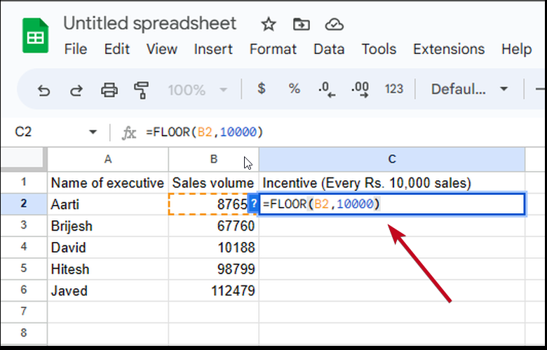
So, we can use the FLOOR function here to find the slab, and hence determine the incentive for Example 1.
That way we can find out how to use the FLOOR function to find the lower closest multiple of an input.
If you have the values in the cells of column B, and we want to get the results in column C, the formula in cell C2, will go as follows.
=FLOOR(B2,10000)
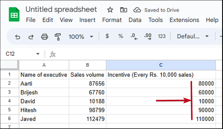
Here, in cell C2, you will get the lowest multiple of 10000, which is close to the number in cell B2.

Just paste the same formula in the subsequent cells of column C, replacing B2 with B3, B4, and so on.

Using the CEILING function (to round down values)
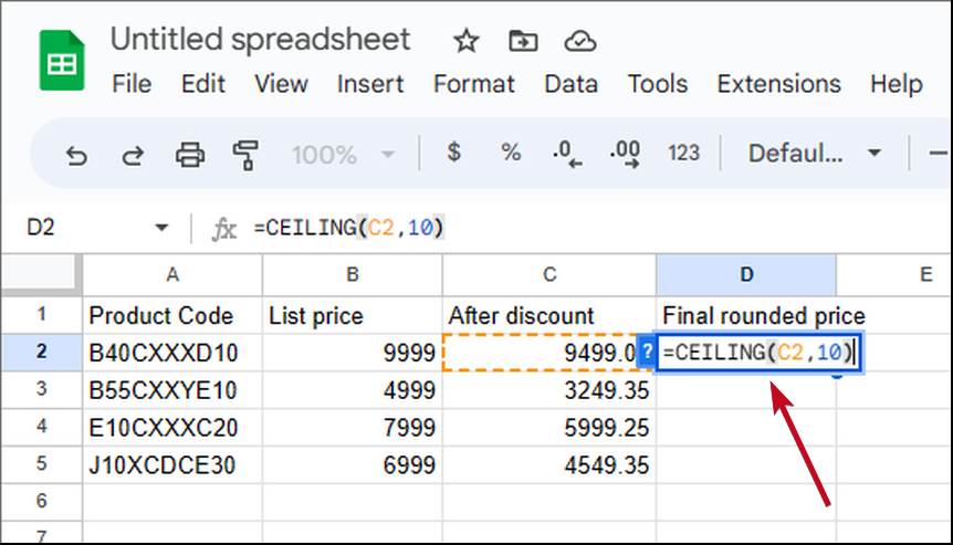
Following Example 2, if we want to find the discounted prices by rounding the calculated value to the upper multiple of the significance, the CEILING function can be used, where we will get the approximate values in column D using the discounted prices in column C.
So, the formula in cell D2 will go as follows.
=CEILING(C2,10)

Replace C2 with C3, and C4 in the subsequent cells in column D.

The FLOOR and the CEILING are the two important functions that you should definitely know and implement if you regularly use Microsoft Excel or Google Sheets to deal with large sets of numbers. Both functions are available in MS Excel, Google Sheets, and other popular spreadsheet applications.
So, that’s all about how to find the lowest or highest close multiple of another number, based on the significance using the FLOOR and CEILING functions. Do you have any questions? Feel free to comment on the same below.

Related Posts
How to create email groups in Gmail? Send one email to multiple recipients in a matter of seconds.
Getting the right dashcam for your needs. All that you need to know
How to Install 7-Zip on Windows 11 or 10 with Single Command
How to Install ASK CLI on Windows 11 or 10
How do you install FlutterFire CLI on Windows 11 or 10?
How to create QR codes on Google Sheets for URLs or any other text elements