How to use conditional formatting and get a better visual representation of your data in Microsoft Excel

When it comes to Microsoft Excel or any other spreadsheet program, the term formatting refers to the font style, font size, cell background-colour, and other aspects. The same goes for word processing programs, as well. But, when it comes to conditional formatting, it is something completely different from normal formatting to apply your favourite font colour, background colour and everything else. In the case of conditional formatting, the formatting will be automatically applied as per your configured settings, depending upon the actual values within the cells, which can make things look more pleasing and understandable to somebody looking at the spreadsheet suddenly.

Let me say a few words about conditional formatting. In the case of conditional formatting, you can configure to automatically change the background colour of the cells to red if the value lies between 0 and 30; yellow, if it lies between 31 and 80; and green, if the value is more than 80. So, if you are creating a spreadsheet of the students in a class and their marks, you can easily see, who are unsuccessful, or the students who have scored less than 30, and those who have scored extraordinary, means more than 80, as they will be marked green. That was just an example, however, there are a number of other ways you can use conditional formatting.

So, without any for the delay, let’s get started with conditional formatting and the way you can implement it in your everyday work with Microsoft Excel.

Using conditional formatting in Microsoft Excel

I will try to explain the complete concept of conditional formatting with a single set of data so that it becomes easy for you to understand.

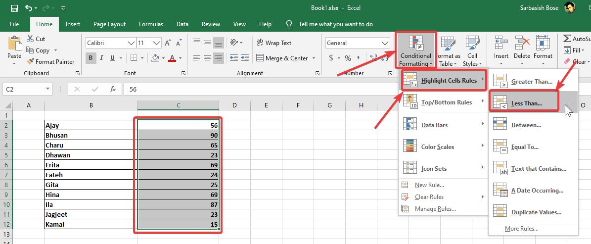
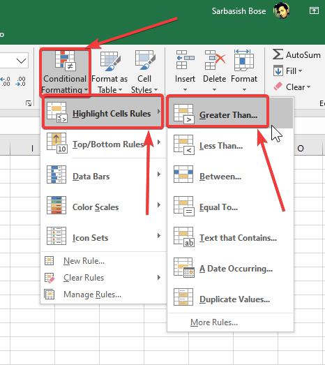
You can find conditional formatting under the home tab in Microsoft Excel, as shown in the screenshot below.

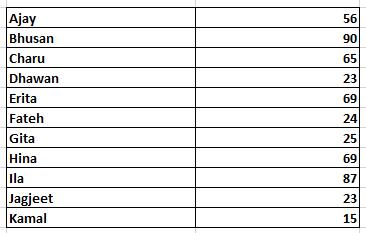
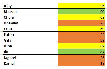
Here is a set of data, which correspond to the marks of 11 students in examination in a particular subject.

First, we will apply the simple rule, which will format the cells containing the marks, in different ways depending upon the marks, in the following way.

The background colours of the cells will be as follows.

0-30: Red

31-80: Yellow

81-100: Green

Conditional formatting as per absolute values

To do that, choose the cells containing the marks, and click on ‘Conditional Formatting’, and choose ‘Less Than…’, under ‘Highlight Cell Rules’.

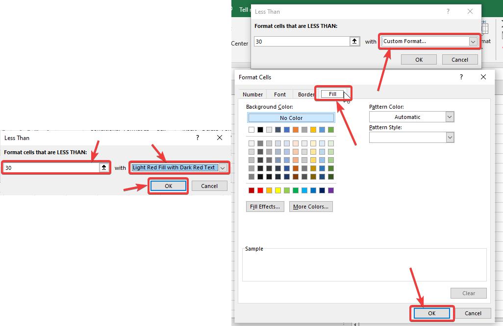
Now, enter 30, under ‘Format cells that are LESS THAN:’, and change the colour from the drop-down menu. Just choose ‘Light Red Fill’, or click ‘Custom Format…’, if you want to apply the exact colour.

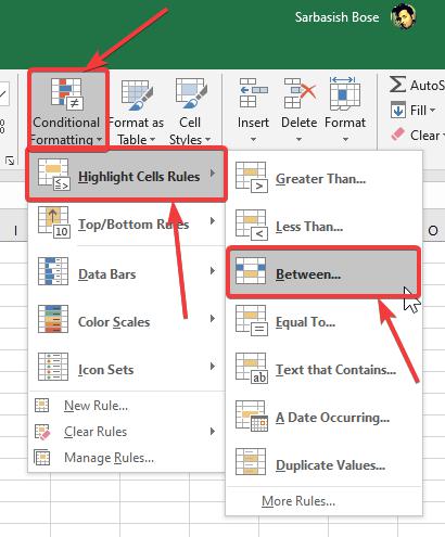
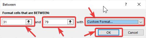
Next, choose the cells again, and click on ‘Between…’, under ‘Highlight Cell Rules’.

Now, enter the range, which will be 31 in the first box and 79 in the next text box. Next, choose a colour close to ‘Yellow’ by choosing ‘Custom Format…’, and finally, click on ‘OK’.

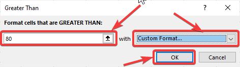
Lastly, Choose the cells again, and click on ‘Greater Than…’ under ‘Highlight Cell Rules’.

Now enter 80 as the value, and choose a gradient of green, from the ‘Custom Format…’ section, and finally, click on ‘OK’.

Now, the conditional formatting is over, and even if you change the values, the colours of the cells are the formatting chosen, will be applied accordingly as per the values updated.

Formatting as per top and bottom rules

Sometimes you might need to format only those cells that contain values more or less than the average of all the values, the top 10 values, the bottom 10 values, the one having the highest and lowest value, or any other similar way.

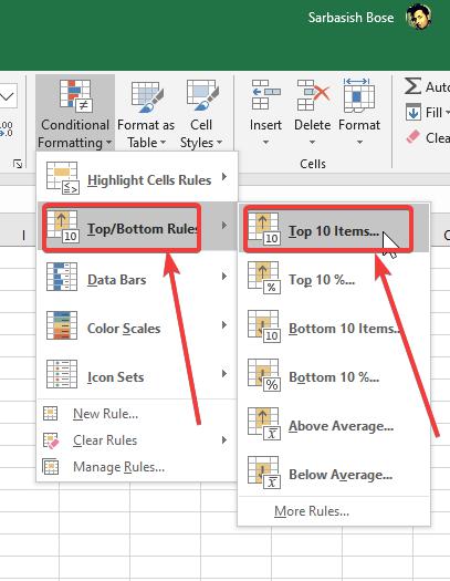
Simply choose ‘Top/Bottom Rules’ under ‘Conditional Formatting’ and choose the appropriate option, that goes as per your requirements.

Here I am formatting only those cells that have the top 10 values.  Simply click on ‘Top 10 Items…’ under ‘Top/Bottom Rules’ under the ‘Conditional Formatting’ option.

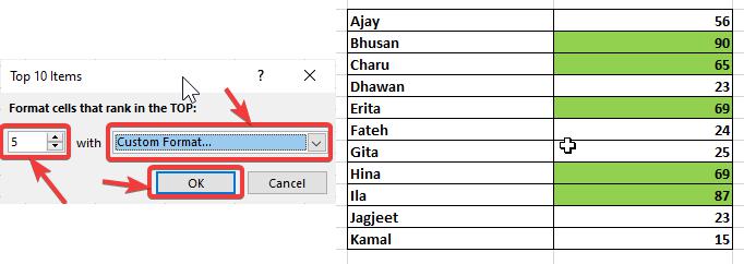
Now, you can choose how many values will be highlighted. By default the value will be set to 10, however, if you change the value to 1, only the cell having the highest value will be highlighted.

Now, you have to change the cell formatting, which includes the font colour, background colour, exactly the same way, we did earlier, in the case of conditional formatting as per the content of the values within the cell.  After you are done, simply click ok to ‘Apply’ the conditional formatting settings.

I have decided to change the background colour of the cells having the top five values with the colour green.

Applying data bars for the cells

You can even show small graphs depending upon the value of the cells. After the implementation, you can understand what I mean to say.

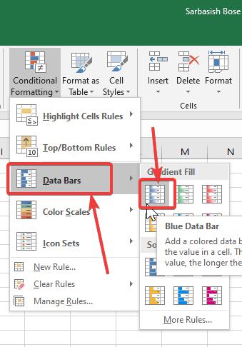
Choose the cells containing the values, and click on any option under gradient fill or solid fill under ‘Data Bars’ under the ‘Conditional Formatting’ options.

After this type of conditional formatting is applied, you can get the following output on the cell.

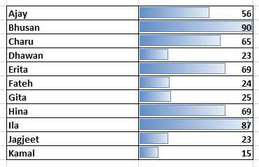
As you can find, there is a small graph having a higher or lower gradient or fill In the cells corresponding to the values. This can also be equally useful if you are having a look at a very big table containing multiple values.

Other conditional formatting options

You can even choose ‘colour Scales’ conditional formatting option, which will automatically assign colours to the cells depending on their values.

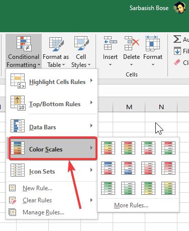
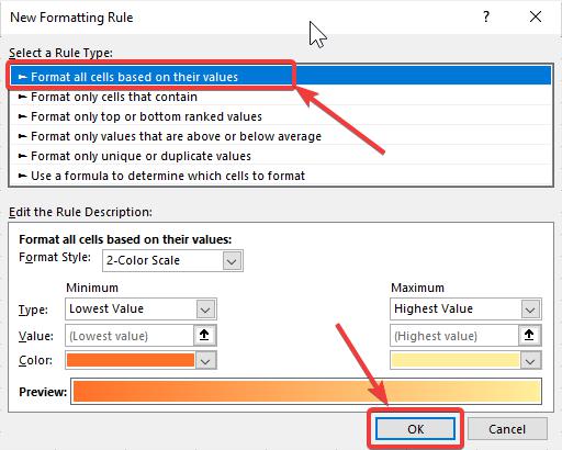
There are already some colour scales, which are ready to be implemented, however, you can even change the values depending upon your requirements, By clicking on ‘More Rules…’ under ‘Color Scales’ in ‘Conditional Formatting’.

Lastly, you can even choose your own set of icons depending upon the values within the cells using the ‘Icon Sets’ option under ‘Conditional Formatting’. You can choose your preferred icon set, depending upon the type of values that you have within the cells, which includes shapes, directional arrows, ratings, and indicators, To suit your needs exactly the way you want. You can even set your own rules, by clicking on ‘More Rules…’ under ‘Icon Sets’.

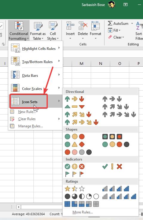
Here’s how it will look, by applying conditional formatting using icon sets.

So, those were the ways you can set up conditional formatting for the values within the cells on Microsoft Excel. The existing rules should cater to the needs of almost all kinds of users, however, you can always choose your new set of rules depending upon the special system requirements, just in case you have one.

Creating a new rule

Just click on ‘New Rule…’ Under conditional formatting, and you have to choose your own set of rules so that the conditional formatting takes place as per your requirement.

When it comes to setting up your new rules, you can choose the most appropriate option depending upon how exactly you want to format the cells depending upon the values.

Changing cells depending upon the value in other cells

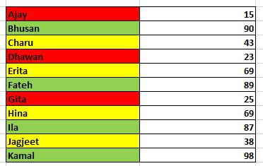
So I talked a lot about how you can change the formatting of the cells depending upon their values. You can also change the formatting of a different set of cells, depending upon the values in another cell.

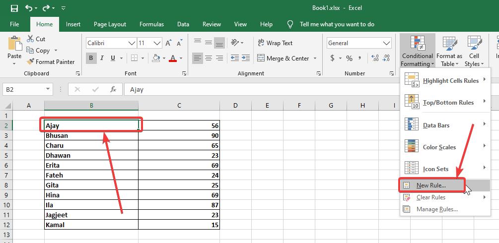
As per the examples, I have discussed here, it is also possible to conditionally format the cells containing the names of students depending upon their marks which are placed on the right side of the cells.

To do that, choose a cell containing the name of a student, (one single cell) and under ‘Conditional Formatting’, click on ‘New Rule…’.

You can find several options here, however, I will choose the option that can help me assign a colour to the students as per their marks, just like the first condition.

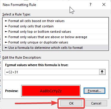
Click on the option that says ‘Use a formula to determine which cells to format’, and enter the formula, corresponding to ‘ Format values where this formula is true:’.

As I have three conditions, I will have to put the first condition here. The background colour of the cells will turn red, if the marks are less than 31, or is between 0 and 30.

So my formula will go as follows.

‘=C2<31’

By clicking on the format option, you can choose the formatting options, which will be a red background for me.

After you are done, click on ‘OK’.

A preview of the cell with conditional formatting when the condition is satisfied will be displayed in the preview section.

Click on ‘OK’ again to apply the conditional formatting settings.

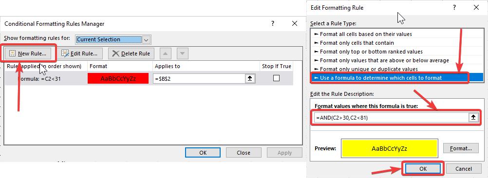
Choose the same cell again, and click on ‘Manage Rules…’ under ‘Conditional Formatting’.

Now, click on ‘New Rule…’, and repeat the same process, I have mentioned in the last step, but the condition will be different for this case.

The condition here will be as below. You can choose the colour as yellow, for the values which are less than 81, but more than 30. So the formula will go as follows.

=AND(C2>30,C2<81)

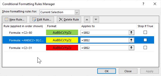
Now you have to go to the same ‘Manage Rules…’ and add another condition that will be ‘=C2 > 80’, and in such a condition, the colour of the cell will turn green.

Once, all the conditions are applied, you can find them all in the ‘Manage Rules…’ under ‘Conditional Formatting’.

After you apply the changes in the first cell, just use the format painter, to copy the formatting of that cell, in the remaining cells containing the names of the students.

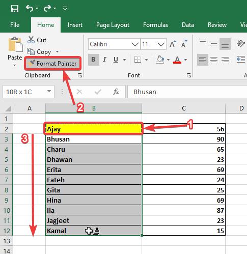
Now the condition will be applied to all the cells, corresponding to the values next to them, and they will be coloured as per the formatting assigned by you.

Conditional formatting is one of the coolest features on Microsoft Excel and other spreadsheet programs available, and once you start learning how to use them, you can unveil other cool tricks while dealing with conditional formatting. After you have formatted your spreadsheet using conditional formatting, you can use the spreadsheet in a slide in a presentation on Microsoft PowerPoint or any other program to create a presentation.

So, that was all about how you can deal with conditional formatting on Microsoft Excel, and deal with their projects in an easier way. Do you have anything else to say? Feel free to comment on the same below.

Other Articles to read:

• How to use VLOOKUP in Microsoft Excel with a basic example
• How to get a Microsoft Excel Worksheet within Microsoft Word
• Tutorial on to create drop-down menus is Google Sheets