How to use VLOOKUP in Microsoft Excel with basic example

From making invoices to maintaining data in a tabular format, Microsoft Excel is undoubtedly the best hub for all such kind of things. Besides that, Microsoft Excel also comes with a ton of formulas, which can definitely come in handy in everyday situations to make your life easier and deal with very big chunks of data, which you might come across if you are maintaining a warehouse, dealing with big data or in similar other situations. Among the different useful functions available in Microsoft Excel, one of them is the VLOOKUP formula of function which can obviously make it easy to deal with enormous data sets.

VLOOKUP is an abbreviation of the term vertical lookup and the term might not be that much self-explanatory and thus, I will discuss it here. To make things easier for you to understand and help you understand the scopes of using VLOOKUP, I will also create a small data set to explain the concept of VLOOKUP. you can, later on, compare the same with big datasets and your imagination that was can be enough to understand how useful it can be, while dealing with big chunks of data in the real world. Even though I will discuss how to use VLOOKUP in Microsoft Excel, you can even use it almost the same way on Google sheets and other office applications.

So without any more delay, let’s get started with what VLOOKUP does.

What is VLOOKUP?

Explaining VLOOKUP in simple terms, it is a lookup formula, which will display the content of a cell in the subsequent columns corresponding to the content of a cell in another column of the same row. I understand things are getting a little confused here.

Let me explain it with an example.

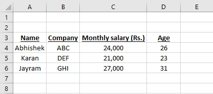
Just consider there are some names of persons in column A and they are present in cells A4, A5, and A6 as shown in the screenshot below.

Now, in B4, B5, and B6, the name of the companies they are working in are written, in C4, C5 and C6, the monthly salaries are mentioned, and finally, in D4, D5, and D6, their ages are written.

Using VLOOKUP in Microsoft Excel or any other office suite application, you can enter the name of the person and get the company they are working in, their salary monthly salary, or their age in a different cell using VLOOKUP.

Thus, here, using VLOOKUP, you can find the company name, monthly salary or age of of Abhishek, Karan or Jayram in any cell, let’s say, in F4, by entering the search keyword, which will be the name in this case, and depending upon, whether we want the company name, monthly salary or age, we can enter the subsequent column number, which will be 2, 3 and 4 for company name, monthly salary and age effectively.

Here, I have listed the salary of Jayram in cell F4 using VLOOKUP.

So, that was a basic definition of VLOOKUP that you should know about.

Let’s now talk about the VLOOKUP formula, so that you can implement it in your everyday life while working with data sets.

Tutorial for VLOOKUP formula with examples

The formula for VLOOKUP goes as follows.

=VLOOKUP(Search_value,table_range,index_number,[match])

Search_value: With respect to the above example, the values are returned, with respect to the name, and thus, it is the search value. If the search value is a string, keep it within double quotes (“ ”).

Table_range: This is the range of the table, which will be searched for the value. VLOOKUP will not lookup for any data outside the given range.

Index_number: It is the row number, corresponding to the search value. It begins from 2, which is the cell that is horizontally next to the first cell. If you enter 1 here, the content of the cell within the first row, which will be ‘name’, as per the above example, will be returned.

[match]: This is optional. Upon entering FALSE, it will search for the exact match, and with the value TRUE, an approximate match will be searched for. If you don’t enter the argument, TRUE is applicable by default.

In the search value argument, you can even enter the cell address, to return the value with respect to the content of that particular cell.

Let’s now make the above example, a little more interesting, where we will find the company name, monthly salary, and age, in H4, H5 and H6 respectively, corresponding to the name entered in H3.

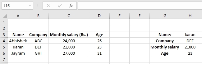
So, the VLOOKUP formula for the cells H4, H5, and H6 respectively will be as below.

H4=VLOOKUP(H3,A4:D6,2, TRUE)

H5=VLOOKUP(H3,A4:D6,3, TRUE)

H6=VLOOKUP(H3,A4:D6,4, TRUE)

As we will enter the name in H3, all the searches will be made corresponding to H3, and thus, H3, the cell address is the search value here.

Next, our table range is from A4 to D6, and thus, the table range is the same in all the cases.

Finally, columns 2, 3, and 4 have the company name, monthly salary, and age respectively, and thus, they are kept as the index number.

I have kept only three names here. But in real life, this 3 can be 3,000, 30,000 or can even be 3 million. Who knows! Searching for data manually in such a big data set isn’t a child’s play, and not even a big man’s play as well. You like to spend hours searching for single data just think how much it will affect your productivity. It is a small example of lookup, that I have mentioned here but it also has support for different other functionalities and you can even deal with multiple sheets and workbooks at the same time.

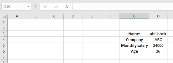
Now, let’s find out, what you have to do if your data is present in a particular sheet, but you want to do VLOOKUP to lookup data from the Sheet 1 and place it in Sheet 2, it could be in Microsoft office or any Apache office and more.

We will use the same example, and instead of finding the company name, monthly salary, and age in Sheet 1, we will find that in Sheet 2.

So, let’s find out how you can do that.

The formula to pull data from another sheet is as given here.

=VLOOKUP(Search_value,’Sheet_name’!table_range,index_number,[match])

Keeping the sheet name in quotes can be useful if the sheet name has spaces in between.

So my formula will go here as follows in Sheet 2, if I want the same values in the same cell addresses, i.e. company name in H4, monthly salary in H5, and age in H6, with respect to the search value in H3.

H4=VLOOKUP(H3,Sheet1!A4:D6,2,TRUE)

H5=VLOOKUP(H3,Sheet1!A4:D6,2,TRUE)

H6=VLOOKUP(H3,Sheet1!A4:D6,4,TRUE)

This is all basic about VLOOKUP in Microsoft Excel, and in the rudimentary level, the following knowledge of VLOOKUP can definitely help to explore the additional possibilities of the function. As Microsoft Excel is not optimized for databases, the performance for searching huge volumes of data might not be as good as searching for the same in some modern database optimized applications. But still, VLOOKUP can definitely come in handy if you are dealing with large sets of data and you have to keep working with legacy systems.

So that was all about the basics of VLOOKUP. Do you have any questions? Feel free to comment on the same below.

Other Articles to read:

• How to get a Microsoft Excel Worksheet within Microsoft Word
• Tutorial to create drop-down menus is Google Sheets to limit the content of a cell
• Insert a picture or text watermark in Excel
• How to find percentage values in Microsoft Excel using the general formula

---