In every Machine Learning problem where there is an association of regression, there is one more term associated and that is called Gradient Descent. As we all know that Linear regression, Logistic regression, SVM, etc. is associated with finding the best fit line to fit in all the points where the slope of the line and bias tend to cover all the points in the dataset. This never happens as a perfect fit line leads to the condition of overfitting. So, the difference that is present between the target output and predicted output is termed as the loss function or the cost function and is given by the difference of predicted value by actual value to the power of 2.
When this cost function is minimum we say that we have attained the point of least error and our model can be used as a benchmark model. In the field of statistics, there is a lot of tuning and tweaking that is done to attain the point of least error.
One of these tweaking processes is updating the weights/slope and biases/intercept. The update of weights and biases in regression-based Machine learning depends upon the cost function, if the cost function of one line is lesser than the other then we will use that line as the best fit line for our problem.
The way we select the values of weights and biases at each update/iteration is achieved with the help of Gradient Descent. The term is frequently used in the field of Data Science. The modern-day Deep Learning algorithms also follow the concept of Gradient Descent. So, what is this Gradient Descent?? Let’s understand this term in detail:
Gradient Descent
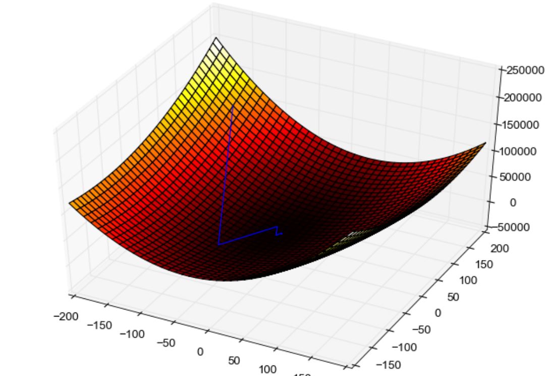
After a person finds the cost function/loss/Sum of squared error concerning the present weight and bias, he will keep on changing the values of weights and biases. These values of bias and Sum of squared error of each line will then be plotted in a graphical form where the y-axis corresponds to the Sum of squared error and the x-axis corresponds to the intercept values. The graph between these two variables represents the shape of an inverted parabola. This parabola comprises a point of minima where the value of error will be the least. To carry out this process manually it requires a lot of time and effort as it is an iterative process but here comes the savior with the name Gradient Descent. With Gradient Descent one can find the point of minimum error very fast and easily.
The mechanism that is adapted by Gradient Descent to speed up the process of weights and bias update is calculating the derivative/slope of the Sum of squared error concerning the bias/intercept. The value of the initial bias is taken to be any random number and then through successive iterations, the Gradient descent algorithm tries to minimize this slope and update the weights accordingly. If the same thing would have been done with the help of just Sum of squared error then the time taken to achieve global minima would have been more and also the proper point of convergence would not have been achieved.
One more thing to note here is that the initial steps that are taken by the Gradient descent algorithms are huge to converge fast but the final steps when it tends to approach the minimum point are small so as not to cross over the minima. The updated weights and biases are achieved with the help of one more parameter that is multiplied with the slope between cost function and intercepts called the learning rate. This learning rate determines how long or short should we take the steps to get the appropriate weights and biases and the least error. The new bias and weight is therefore the difference of the present weight minus the slope of error and intercept multiplied by the learning rate. The value of learning rate should lie between the range of 0 to 1 as high learning rates may lead to a condition where the least slope will not be attainable and it would tend to oscillate over parabola.
Also, the learning rate should not be so small that the error minimization stops before the minima. So, a Data Scientist should be extra careful while selecting the learning rate to carry out the process of Gradient Descent. When we compare this Gradient Descent with Deep learning then the term that is used is called the Back Propagation and the mechanism remains the same.
So, whenever we are performing regression-based analysis or where there is an association of fitting the best line under a graphical representation then the bottom level mechanism behind the working of these algorithms is Gradient Descent. The formula for this is given below with a pictorial representation of the same:
The formula for Cost Function

The formula for Gradient Descent

Related Posts
AirGo Vision- Solos’ Smart Glasses with AI Integration from ChatGPT, Gemini, and Claude
Rise of deepfake technology. How is it impacting society?
OpenAI’s Critic GPT- The New Standard for GPT- 4 Evaluation and Improvement
Claude 3.5 Takes the Lead- Why It’s Better Than GPT-4
Smartphone Apps Get Smarter- Meta AI’s Integration Across Popular Platforms
Free PDF Analysis Made Easy with ChatGPT